When we study statistics, one big challenge is knowing if one thing really causes another. Many times, two things may change together, but that does not mean one causes the other. This is the difference between correlation and causation.
Why Is Causation Hard to Prove?
In many studies—especially in social sciences like economics or sociology—we do not work in a laboratory. We cannot control everything. This means there are many hidden factors that might affect our results. For example, if we study whether drinking more coffee makes people happier, there might be other things affecting happiness that we did not measure. In statistics, this problem is called endogeneity.
What Causes Endogeneity?
There are three common reasons for endogeneity:
1. Omitted Variable Bias
This happens when we forget to include an important variable in our study. For example, if we look at coffee consumption and happiness without considering a person’s income, our study may be biased. Income can affect happiness (because a higher income might mean better healthcare and a better life) and also affect how much coffee a person drinks (because they can afford more). Leaving out income can lead us to make the wrong conclusions about coffee and happiness.
2. Selection Bias
This bias occurs when the people we study are not chosen randomly. For example, imagine if only happy coffee drinkers answer a survey. Then our study will show a strong link between coffee and happiness, but it might not be true for everyone. The sample is not a good mix of all people, which makes the result unreliable.
3. Reversed Causality
Sometimes we might think that one thing causes another when it is really the other way around. Using our example, it could be that being happy makes people drink more coffee, not that drinking more coffee makes them happier. This confusion makes it hard to tell what really causes what.
How Can We Solve These Problems?
There are a couple of ways to address the problems of endogeneity:
Controlling for Omitted Variables
If you have extra data, you can include important factors like income in your study. By doing so, you can see if coffee still has an effect on happiness once income is taken into account.
Using Instrumental Variables
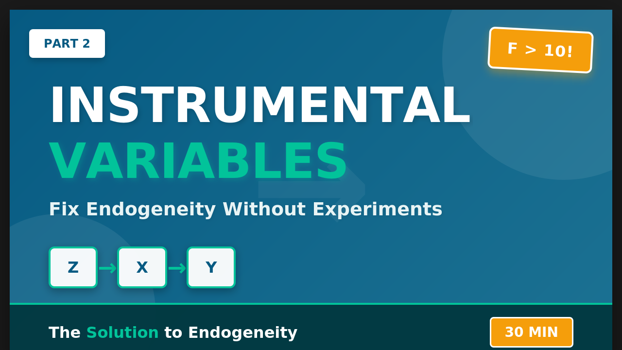
Sometimes, you can use a special variable called an instrumental variable. This is a variable that affects the factor you are interested in (like coffee drinking) but does not directly affect the outcome (happiness).
For example, imagine a company with two departments. In one department, the coffee machine breaks, so people drink less coffee. This broken machine is an external change that is not related to how happy people are. We call this an exogenous shock. Researchers can use this shock to understand the true effect of coffee consumption on happiness.
Creating Statistical Twins
Another idea is to find pairs of people who are very similar in many ways (like income, age, or department) but who drink different amounts of coffee. By comparing these pairs, you can get closer to the true effect of coffee on happiness, almost like doing a mini experiment.
A Sample Dataset for Practice
Below is a simple, fictitious dataset based on our coffee and happiness example. You can use this data to try different statistical methods and see how each one helps in understanding causation.
| ID | Coffee Consumption (cups/day) | Happiness Score (1-10) | Income (dollars) | Department | Machine Status | Survey Participation |
|---|---|---|---|---|---|---|
| 1 | 3 | 7 | 50,000 | A | Working (1) | Responded (1) |
| 2 | 5 | 8 | 70,000 | B | Broken (0) | Responded (1) |
| 3 | 2 | 6 | 45,000 | A | Working (1) | Not Responded (0) |
| 4 | 4 | 9 | 80,000 | B | Broken (0) | Responded (1) |
| 5 | 6 | 8 | 90,000 | B | Broken (0) | Responded (1) |
| 6 | 1 | 5 | 40,000 | A | Working (1) | Responded (1) |
| 7 | 3 | 7 | 55,000 | A | Working (1) | Not Responded (0) |
| 8 | 5 | 8 | 75,000 | B | Broken (0) | Responded (1) |
| 9 | 2 | 6 | 48,000 | A | Working (1) | Responded (1) |
| 10 | 4 | 7 | 65,000 | B | Broken (0) | Responded (1) |
What Does Each Column Mean?
- ID: A number that uniquely identifies each person.
- Coffee Consumption: The number of cups of coffee a person drinks in a day.
- Happiness Score: How happy a person says they are, on a scale from 1 (not happy) to 10 (very happy).
- Income: How much money a person earns in a year.
- Department: Which department the person works in (A or B). In our example, Department B has the broken coffee machine.
- Machine Status: Shows whether the coffee machine is working (1) or broken (0). A broken machine is an example of an external shock.
- Survey Participation: Indicates if a person answered the survey (1 means yes, 0 means no). This helps to see if the group of people responding might be biased.
How to Practice with the Dataset
- Look for Omitted Variables:
Try running a simple analysis of happiness versus coffee consumption. Then, add income to see if the relationship changes. This will help you understand how leaving out important information can change results. - Check for Selection Bias:
Compare the happiness scores of people who responded to the survey versus those who did not. Notice if the group who answered is not representative of the whole group. - Test for Reversed Causality:
Think about whether happiness could be causing more coffee drinking. You might explore methods that look at the order of events (if you have time data) or use techniques to test which way the effect goes. - Use Instrumental Variables:
Try using the machine status (working vs. broken) as a tool (instrument) to see how changes in coffee consumption affect happiness. This method helps to remove the extra problems that come from endogeneity. - Compare Similar People (Statistical Twins):
Find pairs of people in the dataset who are similar in income and department but differ in how much coffee they drink. Compare their happiness scores to see if coffee consumption might be having an effect.
This article explains the main ideas behind causal inference and endogeneity using simple language. The sample dataset gives you a hands-on way to practice and understand these important concepts in statistics. Enjoy exploring these ideas and good luck with your practice!
————————————————–
- Create Sample Dataset for Causal Inference Study *
————————————————–
clear
set more off - Input the dataset
input id coffee happiness income str1 dept machine participation
1 3 7 50000 “A” 1 1
2 5 8 70000 “B” 0 1
3 2 6 45000 “A” 1 0
4 4 9 80000 “B” 0 1
5 6 8 90000 “B” 0 1
6 1 5 40000 “A” 1 1
7 3 7 55000 “A” 1 0
8 5 8 75000 “B” 0 1
9 2 6 48000 “A” 1 1
10 4 7 65000 “B” 0 1
end - Label the variables for clarity
label variable id “ID”
label variable coffee “Coffee Consumption (cups/day)”
label variable happiness “Happiness Score (1-10)”
label variable income “Annual Income (dollars)”
label variable dept “Department (A or B)”
label variable machine “Coffee Machine Status (1=Working, 0=Broken)”
label variable participation “Survey Participation (1=Responded, 0=Not Responded)”
————————————————–
- Explore the Data
————————————————–
describe
summarize
————————————————–
- 1. OLS Regression: Effect of Coffee on Happiness *
- (Simple regression without controls)
————————————————–
regress happiness coffee
————————————————–
- 2. OLS Regression with Income as a Control Variable *
- (Addresses omitted variable bias by controlling for income)
————————————————–
regress happiness coffee income
————————————————–
- 3. Instrumental Variable (IV) Analysis
- Using machine status (exogenous shock) as an instrument for coffee consumption.
- We also control for income.
————————————————–
ivregress 2sls happiness (coffee = machine) income
————————————————–
- 4. Matching (Statistical Twins Approach)
- Here we use nearest neighbor matching to compare similar individuals.
- We match on income and department, and see how differences in coffee affect happiness.
- Note: Requires Stata’s teffects command (Stata 14+).
————————————————–
teffects nnmatch (happiness) (coffee income), n(1)
————————————————–
- Optional: Check for Selection Bias
- For instance, compare happiness scores between respondents and non-respondents.
- (In our dataset, we still have happiness scores for non-respondents, but in practice, missing data can be an issue.)
————————————————–
tabulate participation, summarize(happiness) - End of the Do-file


Leave a Reply