R Code Explanation for PSYC 5133 Drill 2

Setting Working Directory

setwd('/Users/YourNameHere/Desktop')

This line sets the working directory (the default folder where R will look for files and save outputs) to the Desktop folder of the user.

Basic Functions

The code introduces several basic R functions:

• sqrt(): Calculates the square root of a value
• seq(): Generates a sequence of numbers
• remove() or rm(): Removes an object from the R environment
• getwd(): Shows the current working directory
• setwd(): Sets a new working directory
• dir(): Lists files in the current directory

Creating and Manipulating Sequences

y <- seq(from = 1, to = 20, by = 1)

This creates a sequence of numbers from 1 to 20, counting by 1, and assigns it to the variable y.

head(y)
head(y, n = 10)
tail(y)

These functions show the first (head) or last (tail) elements of y. By default, head shows 6 elements, but you can specify a different number.

Basic Statistics

mean(y)
median(y)
sd(y)
var(y)
length(y)

These calculate various statistics for y: mean, median, standard deviation, variance, and the number of elements.

Arithmetic Functions

sum(y)
round(5.76)
log(10)

These perform basic arithmetic operations: sum of all elements in y, rounding a number, and calculating the natural logarithm.

Function Nesting and Piping

round(sd(y))
sd(y) %>% round()

These show two ways to perform the same operation: calculating the standard deviation of y and then rounding it. The second line uses the pipe operator %>% from the tidyverse package.

Loading Packages

library(tidyverse)

This loads the tidyverse package, which includes several useful R packages for data manipulation and visualization.

Working with Data Files

heights <- read.table("https://ytliu0.github.io/Stat390EF-R-Independent-Study-archive/RMarkdownExercises/Galton.txt", 
                      header = T,
                      stringsAsFactors = TRUE)

This reads a data file from the internet and stores it in a data frame called heights.

Exploring Data

head(heights)
glimpse(heights)
colnames(heights)
str(heights)

These functions help explore the structure and content of the heights data frame.

Accessing Data in Data Frames

heights$Height
heights %>% select(Height)
heights[2, 5]
heights[1:5, "Height"]

These show different ways to access specific parts of the data frame.

Basic Data Analysis

mean(heights$Height)
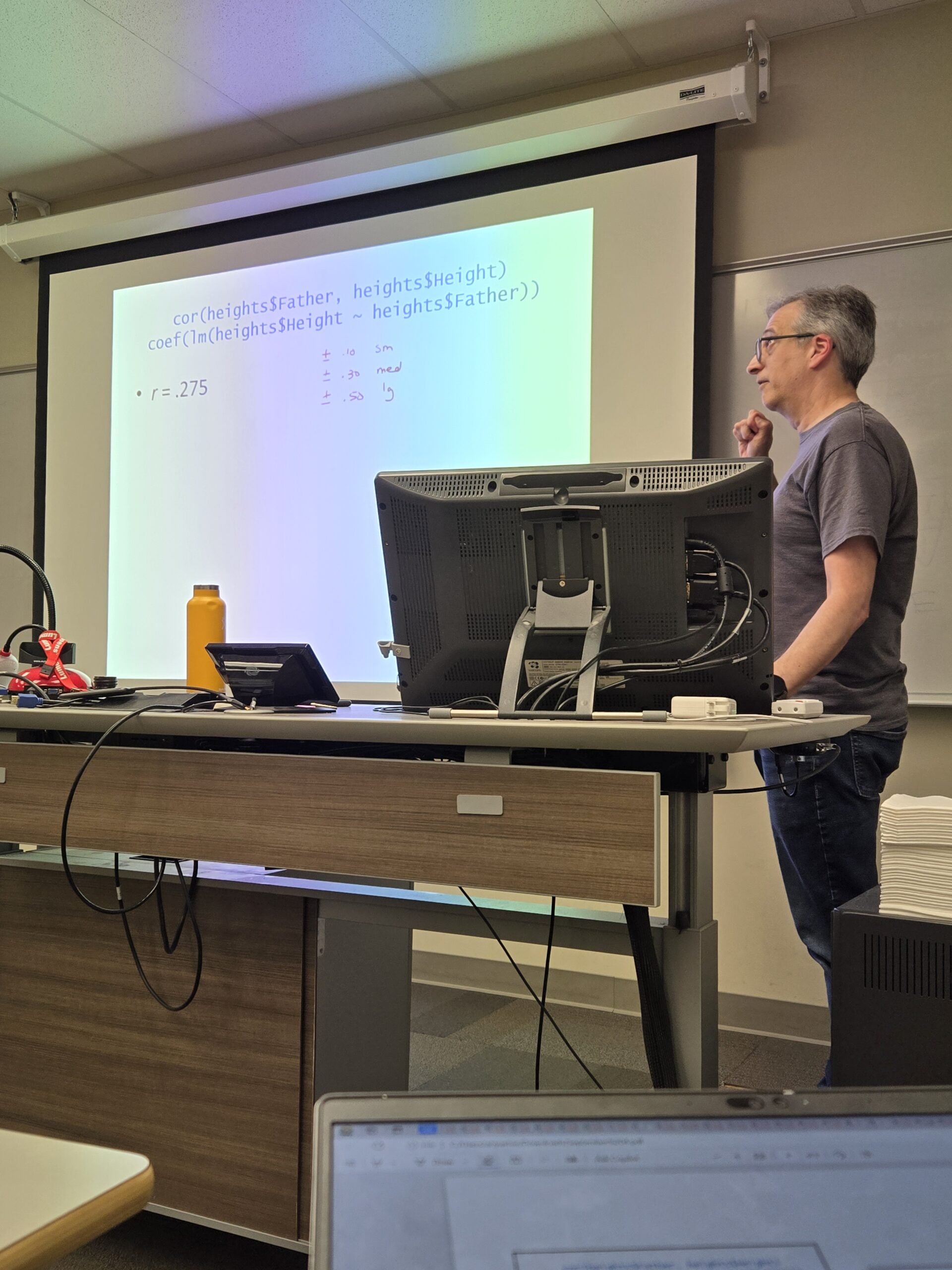
cor(heights$Mother, heights$Father)

These perform basic statistical analyses on the data.

Basic Plotting

hist(heights$Height)
boxplot(heights$Height)
qqnorm(heights$Height)
plot(heights$Father, heights$Height)

These create various types of plots using base R plotting functions.

Advanced Plotting with ggplot2

ggplot(heights, aes(Mother, Father)) + 
  geom_point(position = "jitter") + 
  theme_classic()

This creates a scatter plot using ggplot2, a more advanced plotting package that’s part of tidyverse. It plots Mother’s height against Father’s height, adds jitter to the points, and applies a classic theme to the plot.

This code provides a comprehensive introduction to basic R operations, data manipulation, and visualization techniques.